Plotting lines with error bounds in Matlab
One of my most popular MatlabCentral File Exchange entries is also one of the simplest: boundedline.m. This function allows you to plot confidence intervals (or any other sort of bounds) along the length of a line using a shaded patch object.
Background
Matlab includes the errorbar function to plot error (or standard deviation, confidence intervals, or any sort of bounds) along a line. Here’s one of the examples from the errorbar help page:
count = load('count.dat');

x = (1:size(count,1))';
y = mean(count,2);
e = std(count,1,2);

errorbar(x,y,e,'rx');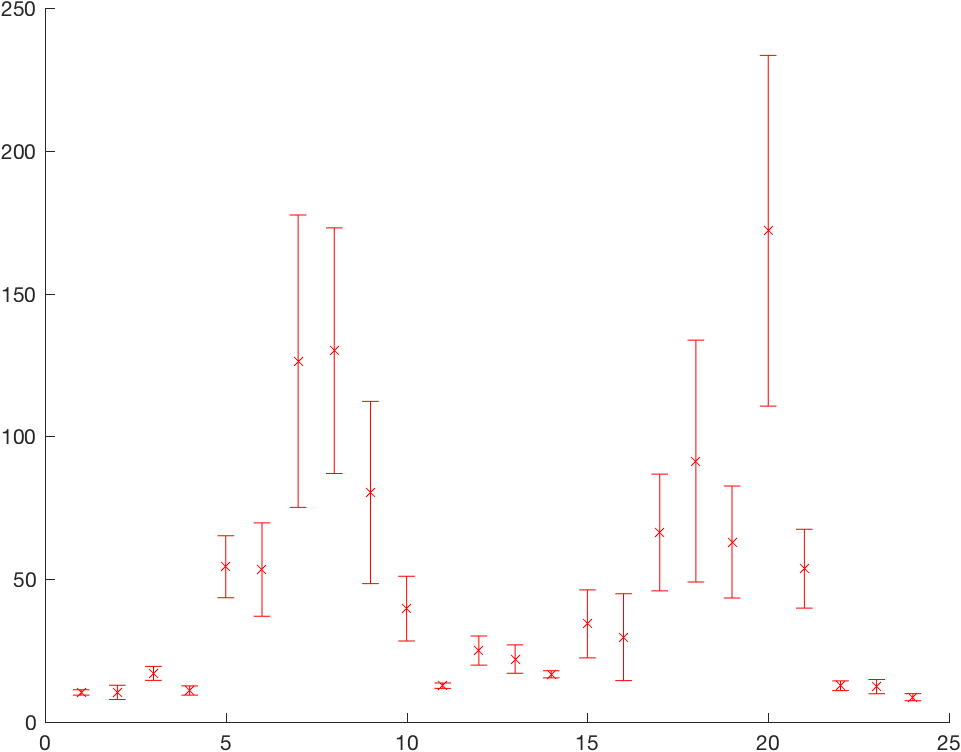
However, often users prefer to visualize error as a shaded region around the line. To get this, you can simply combine the use of a line and a patch. For example:
lo = y - e;
hi = y + e;

hp = patch([x; x(end:-1:1); x(1)], [lo; hi(end:-1:1); lo(1)], 'r');
hold on;
hl = line(x,y);

set(hp, 'facecolor', [1 0.8 0.8], 'edgecolor', 'none');
set(hl, 'color', 'r', 'marker', 'x');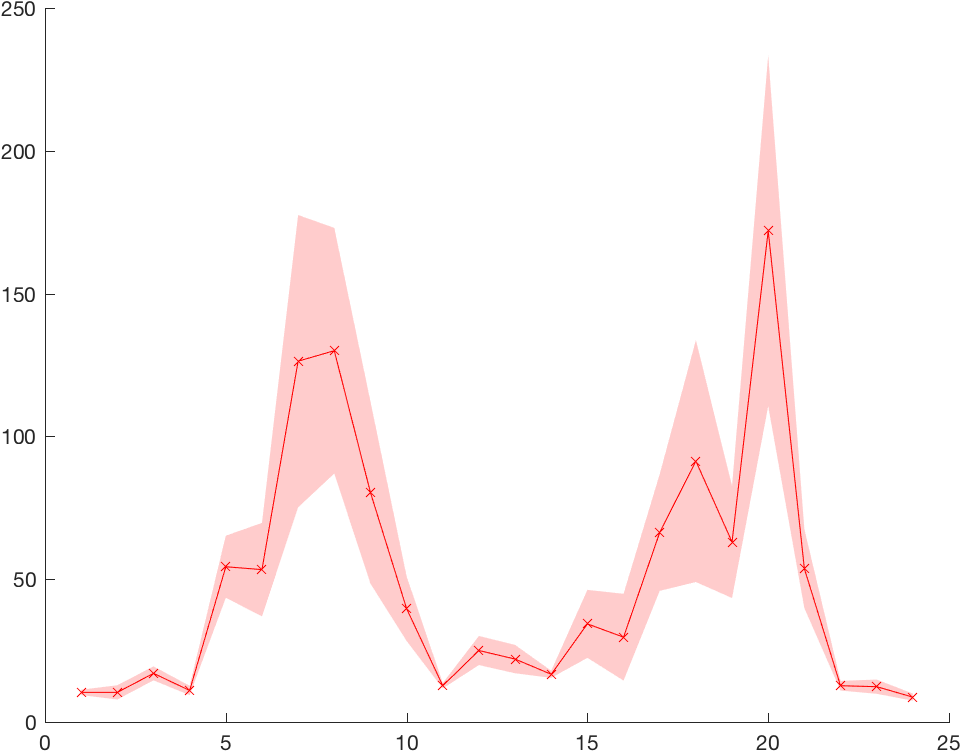
While the concept is simple, keeping all the cosmetic details of the line and patch objects in sync can start to become a hassle if you do this sort of plot a lot. Before I wrote my own function to facilitate the task, I looked at several other candidates on the FileExchange. There were a few features I was looking for in the ideal function:
- It allowed bounds to be set in either the horizontal or vertical direction. In marine sciences, variables are often plotted versus depth, with the y-axis holding the independent variable and the x-axis showing the dependent one.
- It allowed me to plot multiple lines at once.
- It allowed me to specify colors for each line/patch combo.
- It allowed the patch object to be rendered as either the same color as the line, with opacity set to a value less than one, or as an opaque patch colored with a lightened version of the line color. This is less of an issue with the new handle graphics introduced in R2014b, but prior to that, I had a lot of problems with the OpenGL renderer on my computers (OpenGL is the only renderer that supports transparency, but it also led to sporadic visual artifacts that made it unusable for publication-quality graphics); therefore, I needed the option to avoid the use of transparent patches at times.
I didn’t find any candidates that met all of these requirements, so I wrote my own. The boundedline.m function will produce a plot identical to the line/patch combo in the second example above, but with a simpler syntax similar to the errorbar function:
boundedline(x,y,e, '-rx')
The actual plotting function is simple, so instead I focused on making this function as flexible as possible to the types of data one might want to plot. I allow for lots of different calling syntaxes to define one or more lines, similar to the plot function. I also allow several different methods for setting the colors of each line, including the use of LineSpecs, colormaps, or the default color order for an axis. Error bounds can be defined as symmetric on both sides, or you can set different bounds for each side. Bounds can be constant along the length of the line, or vary. Overall, it’s a pretty versatile function, and it’s proved very useful in my own work, and very popular with others as well.
Dealing with NaNs and Infs
One of the more common complaints that I received about this function was that it did not automatically deal with NaNs and Infs in the input data. Line-plotting functions, like plot and line, automatically drop the points,
x = linspace(0,2*pi,100);
y = [sin(x); cos(x); 5*sin(x); 4*cos(x)];
e = rand(100,2,4);

y(randperm(numel(y),5)) = NaN;
y(randperm(numel(y),5)) = Inf;

plot(x,y);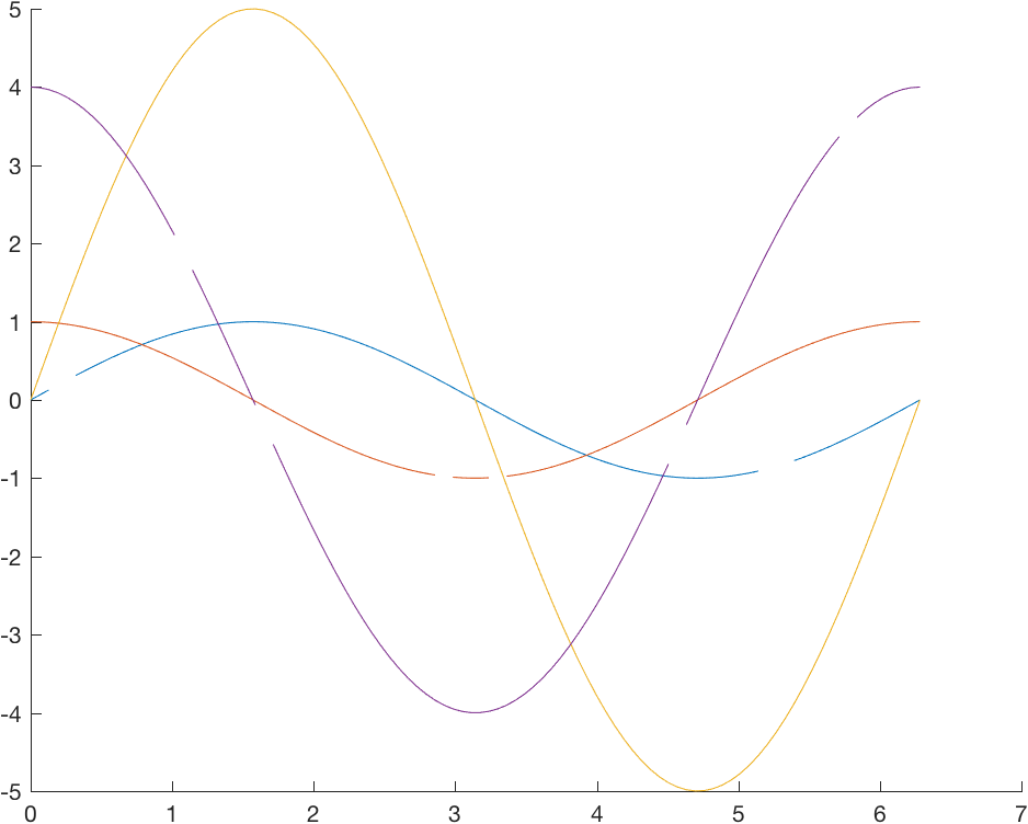
So why couldn’t boundedline do the same?
While dropping the points from the line is pretty easy, figuring out what to do with the patch object is more complicated. Patches do not handle NaNs and Infs gracefully; a patch with a NaN-vertex plots only the outline of the patch, with no fill.
When I asked others what they would expect the function to do when it found NaNs in the patch, the answers varied. Some thought those points should just be dropped from the polygon, interpolating past the NaNs. Others wanted to see a gap in the patch similar to the gap in a line.
When I first wrote this function, I left it up to the users to preprocess their data and remove any NaNs, since there didn’t seem to be a consensus on the desired behavior. I continued to get feedback on this, though, and I recently relented. Now there are three different options for dealing with NaNs included with the boundedline function: drop the points, smooth past them, or leave a gap.
Here’s an example that shows these three methods in action. The markers along the top of the first axis show where I inserted NaNs in the data. Most real datasets won’t include such a variety of missing data, but I wanted to demonstrate behavior in all cases (data missing from the line, data missing from one or both bounds, single missing points vs longer runs of missing data, data missing at the beginning or end of a line, data with 0-width bounds vs missing bounds):
x = linspace(0, 2*pi, 100);
y = sin(x);
e = rand(100,2)*0.2+1;
e(60:65,:) = 0;

ln = [5 12 25:30];
lo = [35 50:55 66:70 95:100];
hi = [40 50:55 66:70];

y(ln) = NaN;
e(lo,1) = NaN;
e(hi,2) = NaN;


nanflag = {'gap', 'fill', 'remove'};
for ii = 1:length(nanflag)
    ax(ii) = subplot(3,1,ii);
    [hl(ii), hp(ii)] = boundedline(x,y,e, 'nan', nanflag{ii});
end
ho = outlinebounds(hl, hp);
set(hl, 'linestyle', ':');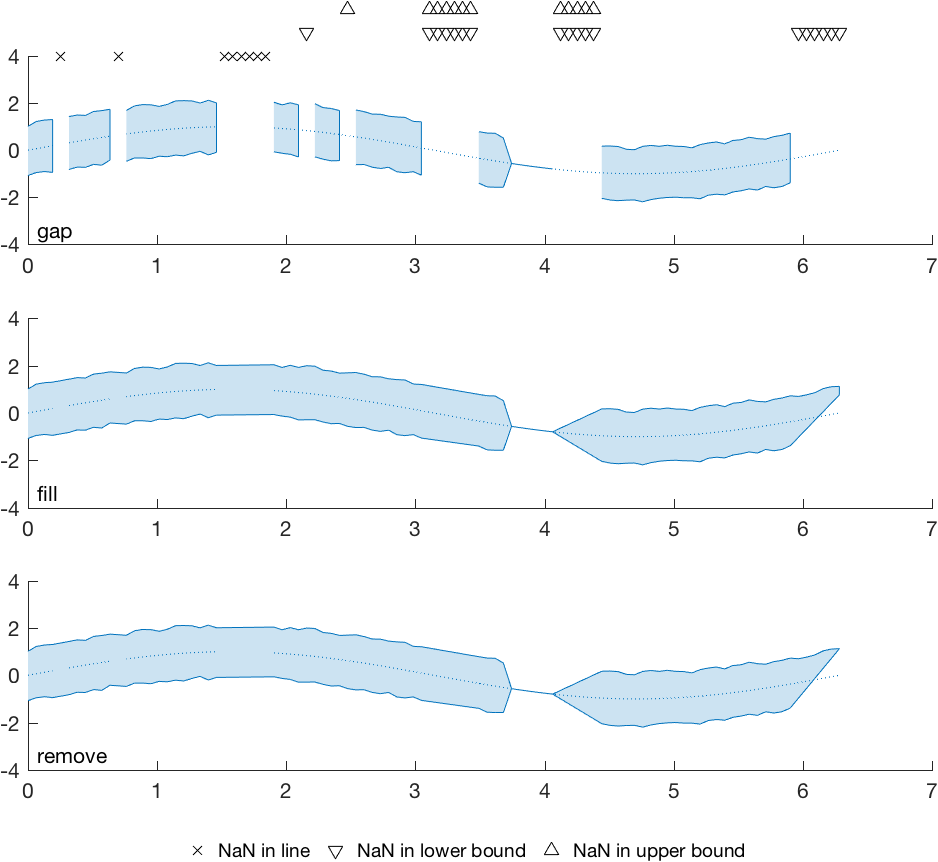
The 'fill' and 'remove' options end up looking the same; the only difference is that the former adds the interpolated points to the patch vertices, while the latter relies on the graphics engine to do this interpolation. You may prefer the former if keeping your vertex numbers consistent with the original data is important for your analysis.
As you can see, the fill/remove option can be a little wonky when you have one-sided missing bounds data at the beginning or end of a line. The gap method is better at highlighting missing data, but it doesn’t differentiate between one-sided and two-sided missing data in the bounds. The fill/remove method may be better if your intent is to mostly ignore a few sporadic missing points in a large dataset (like the missing values on the left side of this example line).
I hope users find that these new NaN/Inf options make this function even more convenient. If you have any additional suggestions for improvement, or want to add a different way of handling gaps, feel free to leave a comment on the File Exchange page for boundedline.m, or raise an issue on the GitHub repo page