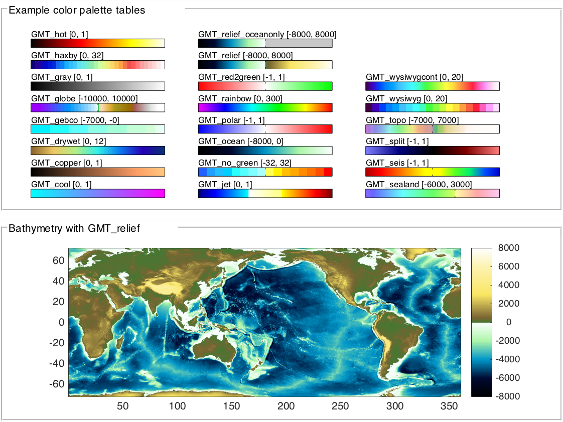
Using color palette tables as Matlab colormaps
I’ll begin my series of Matlab code posts with one of the functions that I use most often in my own work: cptcmap.m.
Matlab comes with a decent selection of colormaps. I was never a fan of the old jet colormap (due to all the inherent issues with rainbow colormaps), but the new parula default is a pretty good general purpose color scheme, and there are several two- or three-color gradients that are also serviceable for publication-quality graphics.
But what are your options when you’re looking for something more specific? What if, like me, you love reading up on color theory and choosing just the right color scheme for each of your plots? The colormapeditor function allows you to play around with custom colormaps, but it’s a very manual process. Particularly when plotting bathymetry and topography data, where I had very specific colors in mind for specific ranges of data, I found myself wishing I could define colormaps more precisely. Early in my career, I used the Generic Mapping Tools software to plot some maps, and while GMT isn’t nearly as user-friendly as Matlab to create quick plots, it certainly produces some beautiful maps. The GMT color palette tables show up in a lot of software used by scientists in oceanography and climate science, such as NASA GISS’s Panoply. And there’s a wonderful assortment of color palette tables available at cpt-city. Why limit myself to a few Matlab colormaps when there are all these options out there?
So a few years ago, while at sea and repeatedly waiting for a CTD to complete it’s two- to three-hour journey to the seafloor and back, I wrote cptcmap.m to import and use GMT-style color palette tables in Matlab.
The color palette file format
The color palette format consists of a simple plain text file:
# COLOR_MODEL = RGB
z0   R0    G0    B0    z1 R1a G1a B1a [A] [;label]
z1   R1b   G1b   B1b   z2 R2a G2a B2a [A] [;label]
...
zn-1 Rn-1b Gn-1b Bn-1b zn Rn  Gn  Bn [A] [;label]
B Rb Gb Bb
F Rf Gf Bf
N Rn Gn Bn
Comments in the color palette file are marked by lines starting with a #. The only comment that isn’t ignored is a comment line that specifies the color model: RGB, CMYK, or HSV. The example above shows the RGB format.
The main color definition section of the file has 8 (RGB, HSV) or 10 (CMYK) columns, plus two optional columns. Each color block is assigned a lower and upper data value (z), and color values to match these bounds. If the lower and upper colors are the same, then that color is assigned to the full range. If the colors are different, then a linear gradient between the two colors results. The optional A flag and semicolon-plus-text column tell GMT how to annotate the color scale. The cptcmap function ignores those optional columns.
The lines begining with B, F, and N indicate the colors used to shade background data values (z < z0), foreground data values (z > zn), and NaN data values, repectively. These three colors aren’t used by cptcmap when creating a colormap, but they can be returned as optional output values.
Converting color palettes to colormaps
The trickiest part of turning a color palette into a colormap is determining the number of colors you need to resolve all the specific color ranges in a given palette. For example:
0  255 0 0  1  255 0 0
1  0 255 0  3  0 255 0
3  0 0 255  6  0 0 255
This color palette is pretty simple: red from 0-1, green from 1-3, and blue from 3-6. To resolve this in a Matlab colormap, you’ll need a 6-color colormap:
1 0 0
0 1 0
0 1 0
0 0 1
0 0 1
0 0 1
with the CLim property of your axis set to [0 6].
By repeating colors in the colormap, you get the appropriate relative size interval for each visible color. This is the primary task of cptcmap; it checks all the color intervals and figures out how many times it needs to repeat colors in order to get all the color breaks in the right place. Once it’s done that, it interpolates the proper number of colors into the new colormap, and (if the direct mapping option is chosen) changes the axis color limits to match the z-values in the color palette table.
Resolution considerations
Under the automated option, I have the number of colors in the final colormap capped at 256. This is the maximum number of colors that can be included on some computers (Windows), and will be more than sufficient for most plots. But you may need to specify a higher number of colors (via the ncol input) if some of your defined color blocks cover a much smaller range than others.
The GMT_globe color palette (one of the GMT defaults, included with cptcmap) demonstrates this resolution problem. I can use the accompanying cptcbar function to compare the discretized colormap to the “real” color palette (the cptcbar on the right uses patches to plot the color intervals, so it is able to resolve everything exactly as it is defined in the color palette; the colorbar on the left shows the actual colormap being used in the figure):
ax = axes;
cptcmap('GMT_globe', 'mapping', 'direct');
cb1 = colorbar('location', 'west');
cb2 = cptcbar(ax, 'GMT_globe', 'east', false);

set([cb1 cb2.ax], 'ylim', [-1500 1500]);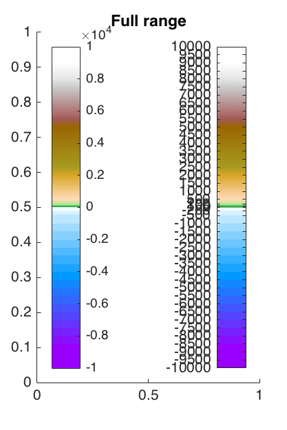
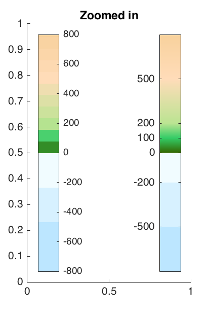
With only 256 colors, we aren’t quite resolving the full color detail intended for low-altitude data. For a global map, this is perfectly acceptable:
[lat,lon,z] = satbath(10);
worldmap('World');
pcolorm(lat,lon,z);
cptcmap('GMT_globe', 'mapping', 'direct');
But zoom in on Florida, and we’re suddenly missing some important detail:
h = usamap('Florida');
[lat,lon,z] = satbath(1, getm(h, 'MapLatLim'), getm(h, 'MapLonLim'));
pcolorm(lat,lon,z);
cptcmap('GMT_globe', 'mapping', 'direct');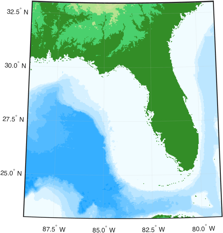
In this case, we’ll want to up the number of colors to resolve all that fine detail in the gradients close to sea level.
cptcmap('GMT_globe', 'mapping', 'direct', 'ncol', 2000);
Limitations
Right now, the cptcmap.m function can read in either RGB or HSV color palette tables. Matlab doesn’t do CMYK-to-RGB conversion natively, and I haven’t actually found any color palette tables that I wanted to use that were defined in CMYK color space, so I simply haven’t gotten around to writing that little conversion yet.